


Next: 4.3.1.1 Generation of stiffness
Up: 4.3 Domain decomposition and
Previous: 4.3 Domain decomposition and
Contents
4.3.1 Non-overlapping elements
Let us assume that our domain  is split into 4 subdomains
each of them was discretized by linear triangular finite elements,
see Fig. 4.5.
is split into 4 subdomains
each of them was discretized by linear triangular finite elements,
see Fig. 4.5.
Figure 4.5:
Non-overlapping elements.
![\begin{figure}\unitlength0.075\textwidth
\savebox{\subdomain} {
\thinlines
\...
...rrow$ ''I''}}
%
\par\end{picture} \ [2ex]
\end{center} \protect\end{figure}](img375.gif) |
We distinguish between 3 sets of nodes denoted by the appropriate subscripts :
- ''I''
- nodes located in the interior of a domain
[
 ],
],
- ''E''
- nodes located in the interior of an interface edge
[
 ],
],
- ''V''
- cross points (vertices), i.e.,
nodes at start and end of an interface edge [
 ].
].
The two latter sets are often combined as coupling nodes with
the subscript ''C'' [
 ].
The total number of nodes is
].
The total number of nodes is
 .
.
For simplification purposes we number first the cross points then
the edge nodes and at last the inner nodes.
The nodes of one edge possess a sequential numbering, the same holds
for the inner nodes of each subdomain so that all vectors and matrices
have a block structure like
According to the mapping of nodes to the  subdomains
![$ \overline{\Omega} \makebox[0pt]{}_i$](img382.gif)
 ,
all entries of matrices and vectors are distributed on the appropriate
process
,
all entries of matrices and vectors are distributed on the appropriate
process
 .
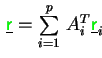
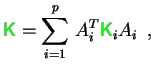
The coincidence matrices
.
The coincidence matrices  (
(
![$ \scriptstyle i=\overline{1,P} \makebox[0pt]{}$](img373.gif) )
represent this mapping.
In detail, the
)
represent this mapping.
In detail, the
 matrix is a boolean matrix
which maps the global vector
matrix is a boolean matrix
which maps the global vector
 onto the local vector
 .
.
Properties of A :
- Entries for inner nodes appear exactly once per row an column.
- Entries for coupling nodes appear once in if this node belongs
to process
.
|
Now, we define 2 types of vectors - the accumulated vector (type I)
and the distributed vector (type-II) :
| Type I |
: |
 und und are stored in process are stored in process
 (
(
![$ \;\hat{=}\;\overline{\Omega} \makebox[0pt]{}_i\;$](img392.gif) ) in the ways ) in the ways
 and
and
 ,
i.e., each process
owns the full values of that vector. ,
i.e., each process
owns the full values of that vector. |
| Type II |
: |
 are stored in the way are stored in the way
 in
such that in
such that
 holds,
i.e., each node on the interface ( holds,
i.e., each node on the interface (
 )
owns only a its contribution
to the full values of that vector. )
owns only a its contribution
to the full values of that vector. |
Matrix  is stored in a distributed way, analogously to a type-II
vector, and will be classified as type-II matrix :
is stored in a distributed way, analogously to a type-II
vector, and will be classified as type-II matrix :
 |
(4.1) |
with
 denoting the stiffness matrix belonging to
subdomain
(to be more exact: the support of the
f.e. test functions is restricted to
).
If one thinks of
as one large finite element then
the distributed storing of the matrix is equivalent to the presentation
of that element matrix previously to the f.e. accumulation.
denoting the stiffness matrix belonging to
subdomain
(to be more exact: the support of the
f.e. test functions is restricted to
).
If one thinks of
as one large finite element then
the distributed storing of the matrix is equivalent to the presentation
of that element matrix previously to the f.e. accumulation.
The special numbering of nodes implies the following
block representation of equation
 :
:
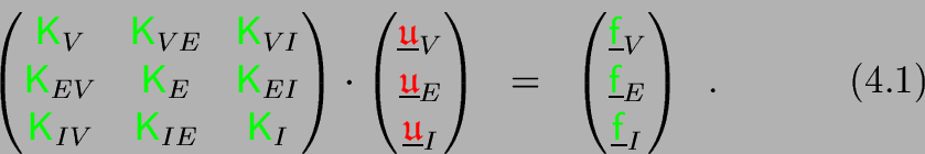
Therein,
 is a block diagonal matrix with
entries
is a block diagonal matrix with
entries
 - similar block structures are valid for
 ,
,
 ,
,
 ,
,
 .
.
If we really perform the global accumulation of matrix
 then the result is a type-I matrix
 and we can write
 |
(4.2) |
Although
 holds,
we have to distinguish between both representations because of
the different local storing (
holds,
we have to distinguish between both representations because of
the different local storing (
 ) !
) !
The diagonal matrix
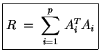 |
(4.3) |
contains for each node the number of subdomains it belongs to
(priority of a node), e.g., in Fig. 4.5
![$ R^{[k]}:=4$](img415.gif) ,
,
![$ R^{[n]}=R^{[m]}=R^{[p]}=2$](img416.gif) ,
, ![$ R^{[q]}=1$](img417.gif) .
.
Declaration : We will use subscripts and superscripts in the
remaining section in the following way :
![$ {\ensuremath{\color{green}{\sf v}}}_{C,i}^{[n]}$](img418.gif) denotes the
denotes the
 component
(in local or global numbering) of vector
component
(in local or global numbering) of vector
 stored in
process
.
Subscript ''
stored in
process
.
Subscript '' '' indicates a subvector belonging to the interface.
A similar notation is used for matrices.
'' indicates a subvector belonging to the interface.
A similar notation is used for matrices.
Subsections
Next: 4.3.1.1 Generation of stiffness
Up: 4.3 Domain decomposition and
Previous: 4.3 Domain decomposition and
Contents
Gundolf Haase
2000-03-20