7.1.2 Sequential solving

To discretize (7.1) in time, the 2-level weighted difference scheme with $L$ as elliptic part of the operator leads to

$$\frac{y(t_{K+1})-y(t_K)}{t_{K+1}-t_K} + \sigma L(y(t_{K+1})) + (1-\sigma) L(y(t_{K})) \;=\; \sigma f(t_{K+1}) + (1-\sigma) f(t_K) \enspace.$$

Choosing $\sigma = 0$ we get the explicit scheme (stability !!),
choosing $\sigma = 1$ results in a purely implicit scheme and
choosing $\sigma = \tfrac{1}{2}$ is the Crank-Nicolson scheme.

3-level difference schemes are also applicable.

If we denote by

 
$\tau=t_{K+1}-t_K$ -- convection matrix  
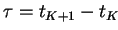
$\tau=t_{K+1}-t_K$ : 		 time step 

$M$ : 		 mass matrix 		 
$\longleftarrow\;\; (u,v)_{L_2}$ 
$\longleftarrow\;\; u$ 

$D$ : 		 diffusion matrix 		 
$\longleftarrow\;\; a(u,v)$ 
$\longleftarrow\;\; \Delta u$ 

$C(u)$ : 		 convection matrix 		 
$\longleftarrow\;\; b(u,u,v)$ 
$\longleftarrow\;\; (u\cdot\nabla) u$ 

$B$ : 		 gradient matrix 		 
$\longleftarrow\;\; (p,\nabla \cdot v)$ 
$\longleftarrow\;\; \nabla p$ 

$B^T$ : 		 divergence matrix 		 
$\longleftarrow\;\; (q,\nabla \cdot u)$ 
$\longleftarrow\;\; \nabla\cdot u$ 


$\underline{u}^K = \underline{u}(t_K)$ : 		  velocity vector 


$\underline{p}^K = \underline{p}(t_K)$ : 		  pressure vector, 

then the discretization in space produces a series of non-linear, non-symmetric and indefinite systems of equations ( $K=0,1,\ldots$) :

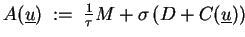
$$\begin{pmatrix}\tfrac{1}{\tau} M + \sigma \left( D + C(\underline... ...\; \begin{pmatrix}\underline{\widehat{f} \makebox[0pt]{}} \ 0 \end{pmatrix}$$ (7.4)

with

$$\underline{\widehat{f} \makebox[0pt]{}} \;:=\; \sigma \underline{... ...ma) \left( D + C(\underline{u}^{K}) \right) \right] \underline{u}^K \enspace.$$

This idea changes $C(\underline{u}^{K+1})$ to $C(\underline{u}^{K})$ in (7.4) (resulting system is called discrete Oseen equations) and together with the definition

$$A(\underline{u}) \;:=\; \tfrac{1}{\tau} M + \sigma \left(D+C(\underline{u})\right)$$ (7.5)

the fix point iteration can be used for solving (7.4).

Using the abbreviations

$$A := A(\underline{u}^n)$$

$$\underline{r} := \underline{\widehat{f} \makebox[0pt]{}} - A(\underline{u}^n) \underline{u}^n - B\underline{p}^n$$

$$\underline{s} := - B^T \underline{u}^n$$

one can write the linear saddle point problem (7.6) in the way

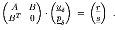$$\begin{pmatrix}A & B \ B^T & 0 \end{pmatrix} \cdot \begin{pmatr... ...x} \;=\; \begin{pmatrix}\underline{r} \ \underline{s} \end{pmatrix} \enspace.$$ (7.6)

The description of properties of $A$ follows closely John [Joh97], pp. 30 :

• Stokes (7.3) $\quad\Longrightarrow\quad$ $A$ symmetric and positive definite.
• Navier-Stokes (7.2) using stabilization by means of sharp upwind or Streamline-Diffusion-Upwind-Petrov-Galerkin (SUPG)
  $\quad\Longrightarrow\quad$ $A=A(\underline{u})$ is regular (i.e., $\exists A^{-1}$), if $u(x)$ fulfills the mass conservation $\nabla\cdot u(x)=0$.
  In certain cases (no obtuse-angled triangles in the mesh) the scheme results in an M-Matrix for $A$ extending the set of applicable solvers considerably.
• Unsteady Navier-Stokes (7.1) $\quad\Longrightarrow\quad$ $A=A(\underline{u})$ is regular if the time step $\tau$ is small enough (stability of the time scheme).
  
  

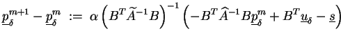
We use the pressure correction scheme for solving (7.7) which is in some way similar to the SIMPLE scheme and the Schur-complement method [Zul97].
Idea : Factor the block matrix $A$ and approximate submatrices to invert :

$$\begin{pmatrix}A & B \ B^T & 0 \end{pmatrix} \approx \begin{pm... ...egin{pmatrix}\widehat{A} \makebox[0pt]{} & B \ 0 & I \end{pmatrix} \enspace,$$

with $\widehat{A} \makebox[0pt]{} \approx A$ and $\widehat{C} \makebox[0pt]{} \approx B^T A^{-1} B$ approximates the negative Schur-complement.
Here and in the following, we denote by $G\approx H$ the spectral equivalence between matrices $G$ and $H$ possessing the same rank $n$, i.e, there exist positive constants $\underline{c}$, $\overline{c}$ so that

$$\underline{c} \left( G\cdot\underline{v} , \underline{v} \right) ... ...v} \right) \qquad\forall \underline{v} \in \ensuremath{\mathbb{R}}^n \enspace.$$

Remarks :

1. Deleting the third line in algorithm 7.2 results in the preconditioned Arrow-Hurwicz algorithm
   
   
   

   

   
   
2. If one chooses $\widehat{C} \makebox[0pt]{} = \tfrac{1}{\tau} I_{N_p}$, $\widehat{A} \makebox[0pt]{}=A$ and deletes the third line in algorithm 7.2 we get the classical Uzawa algorithm [BF91]. Its iteration matrix is symmetric with respect to a special chosen inner product.
   
   
   

   

   
   
3. For solving the pressure correction (7.8) as accurate as possible often the fix point iteration

   $$\underline{p}^{m+1}_{\delta} - \underline{p}^{m}_{\delta} \;:=\; ... ...\underline{p}^{m}_{\delta} + B^T \underline{u}_{\delta} - \underline{s} \right)$$ (7.7)

   
   
   is used with $\widetilde{A} \makebox[0pt]{} \approx A$.
   Admissible matrices for $\widetilde{A} \makebox[0pt]{}$ : Identity $I_{N_u}$, mass matrix $M$ (non-conform elements), $\mathrm{diag}(A)$.
   Possible choices for $\left(B^T \widetilde{A} \makebox[0pt]{}^{-1} B \right)$ : Identity $I_{N_p}$, mass matrix $M_{N_p}$ (diagonal matrix if test functions for the pressure are constant per element).
   In the symmetric case, the matrix $B^T \widetilde{A} \makebox[0pt]{}^{-1} B$ is positive semidefinite (i.e., all eigenvalues are greater or equal 0). By fixing one component of $\underline{p}_{\delta}$ the related system of equations (7.9) can be solved via some proper iteration method (gmres, cg, mg). Therein, instead of the inverse of $B^T \widetilde{A} \makebox[0pt]{}^{-1} B$ only the multiplication of that matrix with a vector is needed.
4. Usually, also $\widehat{A} \makebox[0pt]{}^{-1}$ will be realized via an iteration method.
5. The fix point iteration (algorithm 7.1) was derived by a linearization of (7.4) using
   $$C(\underline{u}^{K+1}) \underline{u}^{K+1} \quad\xrightarrow[\ma... ...t}]{\mathrm{linear}} \quad C(\underline{u}^{K}) \underline{u}^{K+1} \enspace.$$
   On the other hand, the substitution
   $$C(\underline{u}^{K+1}) \underline{u}^{K+1} \quad\xrightarrow[\ma... ...}]{\mathrm{convection}} \quad C(\underline{u}^{K}) \underline{u}^{K} \enspace,$$
   leads directly to the saddle point problem (7.7) with the components
   

   $$A := \tfrac{1}{\tau} M + \sigma D$$

   $$\underline{r} := \sigma \underline{f}(t_{K+1}) + (1-\sigma) \underline{f}(t_K) + \... ...\tfrac{1}{\tau} M - (1-\sigma) D - C(\underline{u}^{K}) \right] \underline{u}^K$$

   $$\underline{s} := 0 \enspace,$$

   
   
   which produces the solution $\underline{u}^{K+1}:=\underline{u}_{\delta}$, $\underline{p}^{K+1}:=\underline{p}_{\delta}$.
   If there is a dominating convective part in the differential equation then this scheme may run into stability problems (in the time integration) due to the explicit handling of the convection.
6. The stationary Navier-Stokes equations (7.2) are represented by (7.4) with the components
   $$M:=0 \enspace,\qquad\sigma:=1 \enspace,\qquad \underline{u}:=\und... ...enspace,\qquad\underline{p}:=\underline{p}^{K+1}\:=\underline{p}^{K} \enspace.$$

7. The Stokes equations (7.3) are just the saddle point problem (7.7) with
   $$A:=D \enspace,\qquad\underline{r}:=\underline{f}\enspace,\qquad s... ...ine{u}_{\delta} \enspace,\qquad\underline{p}:=\underline{p}_{\delta} \enspace.$$
   Matrix $A$ is symmetric and positive definite (spd).