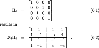
A rearranging of the entries in (6.9) by means of the
permutation matrix
From
and the
definition
diag
follows immediately
(6.10)
i.e., the Fourier analysis for is defined by the Fourier analysis for .
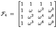
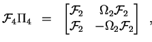
Generally :
For we have
(6.11)
with as an even-odd permutation
which rearranges the vector components
(6.12)
and
diag.
If holds, then formula (6.13) can be applied
recursively times
so that the FFT will be reduced to rearrangements of vectors with only
little additional arithmetics.
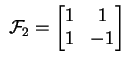
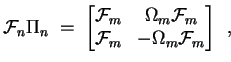
FFT with
In the remaining section, denotes that subvector of
which contains from element 0 to element each second
component, i.e.,
Figure 6.7:
Split of subscripts
The rearrangement in Fig. 6.7 results in
a vector
.
Fig. 6.8 presents the so called
butterfly algorithm
which is a parallel realization of the Fourier transformation
(arithmetics and rearranging)
on a distributed memory computer.
Therein one sees the good parallelization properties of the Fourier
transformation, however the resulting components are present
unordered and their rearranging requires additional communication.
Figure 6.8:
Looking back on the example at the beginning of this section 6.4,
we see that we have to solve the equation
instead of the discrete equation
:
a)
Fourier analysis :
rearranged
b)
Operator
:
rearranged
c)
Fourier synthesis :
in correct order !!
Since the Fourier transformation had to be used twice, the components
of the solution are present again in correct order in the end!
The combination of Fourier analysis and synthesis can be parallelized very well.
 and the
definition
and the
definition
 diag
diag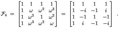
![$\displaystyle \underline{y}\;:=\; \Pi_n^T \underline{x} \quad\Leftrightarrow\qu...
..._j & {\scriptstyle j=\overline{1,n-1:2} \makebox[0pt]{}} \end{bmatrix} \enspace$](img810.gif)
![$\textstyle \parbox{10cm}{Flow chart on 4 processors
\ <I>
The marked bits of ...
...opriate bit
for the next butterfly operation.
[Dr. Pester Chemnitz].
</I>}$](img819.gif)