3.1 Some definitions

Scalability :
Simple (or better automatic) adaption of a program to a given number of processors.

Scalability is meanwhile more highly evaluated than highest efficiency (i.e., gain at computing time by parallelism) on one special architecture/topology.

Granularity :
Size of program sections, which are executable without communication with other processors.

Fine grain algorithm : $\longrightarrow$ systolic arrays [SIMD]

Ex.: $\omega$-Jacobi iteration

Laplace problem, discretized by means of a 5-point stencil.

$$d_{i,j} := c_{i,j} + \left({ f_{i,j} - \omega \left[ - c_{i-1,j} - c_{i,j-1} + 4 c_{i,j} - c_{i+1,j} - c_{i,j+1} \right] }\right) / 4$$

$$\underline{c} := \underline{d}$$

Here, no data dependencies occur within one iteration.
$\Longrightarrow$ easy to parallelize (and vectorize).

Ex.: $\omega$-Gauß-Seidel iteration (forward)

Laplace problem, discretized by means of a 5-point stencil.

$$\widehat{c} \makebox[0pt]{}_{i,j} \;:=\; c_{i,j} + \left({ f_{i,... ...akebox[0pt]{}_{i,j-1} + 4 c_{i,j} - c_{i+1,j} - c_{i,j+1} \right] }\right) / 4$$

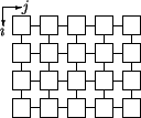
Figure 3.1: Gauß-Seidel on a systolic array

The values $\widehat{c} \makebox[0pt]{}_{i-1,j}$ and $\widehat{c} \makebox[0pt]{}_{i,j-1}$ have to be calculated previously to the calculation of $\widehat{c} \makebox[0pt]{}_{i,j}$.

• Calculation acts like a wave front {1 $^{\text{st}}$ ,2 $^{\text{nd}}$ ,3 $^{\text{rd}}$ ,4tex2html_wrap_inline^th step}.
• $m\times n$ systolic array.
  $\longrightarrow$ it takes ($m+n-1$) time cycles for one iteration.
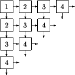
  $\longrightarrow$ A consecutively execution of several iterations compensates this overhead of the startup phase.

1 $^{\text{st}}$ iteration :
Reduction of run time :
$\frac{t_{\text{parallel}}}{t_{\text{sequential}}} = \frac{m+n-1}{mn} \a... ...c{2\sqrt{mn}}{mn} = \frac{2}{\sqrt{mn}} = {\cal O}(\frac{1}{\sqrt{P}})$
An optimal ratio would be $\frac{1}{P} = \frac{1}{mn}$ !

2 $^{\text{nd}}$ iteration :

• It takes the iterations following the startup only one time cycle per iteration. This behavior is similar to the filling of the vector pipes in a vector unit.
• It takes the $k$tex2html_wrap_inline^th (last) iteration the same time as the first iteration. $$\begin{eqnarray*} \textstyle \frac{t_{\text{parallel}}}{t_{\text{sequential}}}... ... \stackrel{k\mapsto \infty}{\longrightarrow} \frac{1}{mn} \end{eqnarray*}$$

This parallelization is asymptotically optimal, i.e., a large number of iterations achieves the best gain at time.

Coarse grain algorithm : $\longrightarrow$ Multiple processor machine [MIMD]
e.g. block variant of $\omega$-Jacobi or Gauß-Seidel iteration

Remark : The communication between processes takes considerably more time than arithmetic operations or accesses to local memory. Thus, coarse grain algorithms are of great advantage in parallelization of algorithms.

Functional parallelism :
Splitting of an algorithm into parallel executable tasks which realize different operations on the data.

Ex.: $E = (d \ast e \ast f + g + c) \ast b + a +h$

• sequential (from left to right) 7 clocks
• parallel on 2 processors 5 clocks
  
  

  Figure 3.2: Functional parallelism on 2 processors/units

  

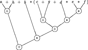Exercise 8:

Distribute the operations above on 3 processors.
Hint : Use arithmetic transformation rules (result: 4 clocks).

• A parallel algorithm may contain more arithmetic operations, nevertheless this algorithms is (at least theoretically) faster than the sequental one.
• Functional parallelism contains only a limited scalability. In the example above, the use of more than 3 processors would not lead to a further decrease in execution time.

Data parallelism :
One part (or similar parts) of a program are executed in parallel on different sets of data.

• Prerequisite: Simple splitting of data into blocks (High Performance Fortran).
• It is (relatively) easy to scale. Problems occure in case of more complicated data dependencies like indirect addressing (FEM).

Ex.: Block-$\omega$-Jacobi

• Distribution of vectors and matrices.
• Several opportunities for distribution (see Sec. 5)

Special case : Geometric parallelism.

The set of data is split into subsets with respect to geometric relations of the objects of interest (nodes of discretization, particles, ...). These relations are represented in the matrix graph in case of a FEM,FDM or FVM discretization.