Contents
- CompMath-Vorlesung 08.10.2021
- Symbolische Ausdruecke
- Symbolische Funktionen
- Manipulation algebraischer Ausdruecke
- Ausdrücke vereinfachen
- Algebraische Gleichungen
- Loese nach der einzigen Variablen auf: symbolisch
- Loese symbolisch mit Zusatzannahme
- Loese nach einer bestimmten Variablen symbolisch auf ("Umstellen nach")
- Schraenke das Loesen auf x>0 ein.
- Loese nach der einzigen Variablen auf: numerisch mit vpasolve()
- Loese nach der einzigen Variablen auf: numerisch fzero()
- Algebraische Gleichungssysteme
- Lineares System
- Variante 1: symbolisch (mit Parameter) via solve()
- Variante 2: numerisch via \
- Nichtlineares System
- Variante 1: symbolisch via solve()
- nochmal symbolisch, aber mit Parameter in Loesung via solve()
- numerische Loesung via vpasolve()
- numerische Loesung via fsolve() [benoetigt die Optimization Toolbox]
- Integrieren und Differenzieren nach einer Variablen
- Int+Diff+Vereinfachen
- Integrieren und Differenzieren mehrdimensionaler Funktionen
- Gradient, Laplace, Rotation, Divergenz
- Grenzwerte:
- Evaluate the sum of the following multivariable expression with respect to k:
- Grafik mit symbolischen Funktionen
- Visualisierung mit 2 Variablen (nur mit Funktion moeglich)
CompMath-Vorlesung 08.10.2021
Demonstration symbolischer Methoden in Matlab, Siehe auch die gute Einfuehrung dazu.
close all;  clear; clc

% Präambel für Octave
isOctave = exist('OCTAVE_VERSION', 'builtin') ~= 0;
if (isOctave)
   pkg load symbolic                         % nur fuer octave noetig
end
Symbolische Ausdruecke
clear
disp('Symbolische Ausdruecke');
%  Deklaration
syms a b c;        % deklariere symbolische Variablen
f = 3*(a-1)*(b^2+c^3)*(exp(a+b)-1)   % symbolischer Ausdrücke

% Ersetzen von Variablen durch Zahlenwerten oder Ausdruecke
subs(f, a, 3)              % Ersetze a durch 3
subs(f, a, b)              % Ersetze a durch (bereits als symb. def.) Variable b
subs(f, a, 'x')            % Ersetze a durch (noch nicht als symb.) Variable x
subs(f, a, (b+c)^2)        % Ersetze a durch den Term (b+c)^2
subs(f, [a,b,c], [-1,2,3]) % Ersetze die Variablen durch die Werte/Terme
Symbolische Ausdruecke

f =

(3*a - 3)*(b^2 + c^3)*(exp(a + b) - 1)


ans =

6*(exp(b + 3) - 1)*(b^2 + c^3)


ans =

(3*b - 3)*(exp(2*b) - 1)*(b^2 + c^3)


ans =

(3*x - 3)*(b^2 + c^3)*(exp(b + x) - 1)


ans =

(exp(b + (b + c)^2) - 1)*(3*(b + c)^2 - 3)*(b^2 + c^3)


ans =

186 - 186*exp(1)
Symbolische Funktionen
clear all;

disp('Symbolische Funktionen');
%  Deklaration
syms a b c;        % deklariere symbolische Variablen
f(a,b,c) = 3*(a-1)*(b^2+c^3)*(exp(a+b)-1)   % symbolische Funktion

% Ersetzen von Variablen durch Zahlenwerten oder Ausdruecke
f(3,b,c)              % Ersetze a durch 3
f(b,b,c)              % Ersetze a durch (bereits als symb. def.) Variable b
f('x',b,c)            % Ersetze a durch (noch nicht als symb.) Variable x
f((b+c)^2,b,c)        % Ersetze a durch den Term (b+c)^2
f(-1,2,3)             % Ersetze die Variablen [a,b,c] durch die Werte/Terme
Symbolische Funktionen

f(a, b, c) =

(3*a - 3)*(b^2 + c^3)*(exp(a + b) - 1)


ans =

6*(exp(b + 3) - 1)*(b^2 + c^3)


ans =

(3*b - 3)*(exp(2*b) - 1)*(b^2 + c^3)


ans =

(3*x - 3)*(b^2 + c^3)*(exp(b + x) - 1)


ans =

(exp(b + (b + c)^2) - 1)*(3*(b + c)^2 - 3)*(b^2 + c^3)


ans =

186 - 186*exp(1)
Manipulation algebraischer Ausdruecke
a^2-2*a*b+b^2
clear;
%clc;

disp('Manipulation algebraischer Ausdruecke');
syms a b;         % deklariere symb. Variablen
f = a^2-2*a*b+b^2 % symb. Funktion

fe = factor(f)    % Faktoren bestimmen
prod(fe)          % ausmultiplizieren der Faktoren
Manipulation algebraischer Ausdruecke

f =

a^2 - 2*a*b + b^2


fe =

[ a - b, a - b]


ans =

(a - b)^2
Ausdrücke vereinfachen
disp('simple anwenden')
ff=simplify(f)      % (bestmoeglich) vereinfachen, zeigt alle Versuche
expand(ff)          % ausmultiplizieren der Ausdrücke
simple anwenden

ff =

(a - b)^2


ans =

a^2 - 2*a*b + b^2
Algebraische Gleichungen
Loese x^2=16
Loese nach der einzigen Variablen auf: symbolisch
clear;
%clc;
disp('Loese nach der einzigen Variablen auf')
% Loese x^2=16:  Variante 1
syms x
assume(x,'clear')                   % ensure that all old assumtions are deleted
solve(x^2 == 16)

% Loese x^2=16:  Variante 2
syms x;
y = x^2-16;
solve(y==0, x)       % Loest  y(x) = 0
Loese nach der einzigen Variablen auf

ans =

 -4
  4


ans =

 -4
  4
Loese symbolisch mit Zusatzannahme
clear;
syms x
assume(x,'clear')                   % ensure that all old assumtions are deleted
f = x^4 - x^3 - 5*x^2 - 7*x - 84
disp('Loese ohne Zusatzannahme')
xsol = solve(f==0)

disp('x soll reell sein')
assume(x,'real')
xsol = solve(f==0)

disp('x soll zusaetzlich negativ sein')
assumeAlso(x<0)
xsol = solve(f==0)

disp('assumptions(x) :')
assumptions(x)
f =

x^4 - x^3 - 5*x^2 - 7*x - 84

Loese ohne Zusatzannahme

xsol =

          -3
           4
 -7^(1/2)*1i
  7^(1/2)*1i

x soll reell sein

xsol =

 -3
  4

x soll zusaetzlich negativ sein

xsol =

-3

assumptions(x) :

ans =

[ in(x, 'real'), x < 0]
Loese nach einer bestimmten Variablen symbolisch auf ("Umstellen nach")
Stelle y = 2*x^2+4 nach x um
clear;
%clc;
disp('Loese nach einer bestimmten Variablen auf')
syms x y;
f  = 2*x^2+4-y       %  Notwendig:  f(x,y) = 0
% f = sin(x)-x/2-0.1;
aa = solve(f==0,x)
pretty(aa)
% Schoenere Ausgabe
Loese nach einer bestimmten Variablen auf

f =

2*x^2 - y + 4


aa =

 -(2^(1/2)*(y - 4)^(1/2))/2
  (2^(1/2)*(y - 4)^(1/2))/2

/   sqrt(2) sqrt(y - 4) \
| - ------------------- |
|            2          |
|                       |
|  sqrt(2) sqrt(y - 4)  |
|  -------------------  |
\           2           /
Schraenke das Loesen auf x>0 ein.
assume(x>0)                 % nur positive Lösungen
a1 = solve(f==0,x)          % matlab weist auf Lösungsbedingung hin

assume(4<y)                 % Lösungsbedingung bzgl.  y  festlegen
a2 = solve(f==0,x)
Warning: Solutions are valid under the following conditions: 4 < y. To include
parameters and conditions in the solution, specify the 'ReturnConditions' value
as 'true'.

a1 =

(2^(1/2)*(y - 4)^(1/2))/2


a2 =

(2^(1/2)*(y - 4)^(1/2))/2
Loese nach der einzigen Variablen auf: numerisch mit vpasolve()
syms x;
y = x^2-16;
% y = sin(x)-x/2-0.1;

disp('Numerisch mit  vpasolve():')
x0  = -1;
%
% sol = vpasolve(y)         % funktioniert auch
sol = vpasolve(y, x0)
disp(['Startloesung ', num2str(x0), ' ergibt Lösung: ']);
sol
Numerisch mit  vpasolve():

sol =

 -4.0
  4.0

Startloesung -1 ergibt Lösung:

sol =

 -4.0
  4.0
Loese nach der einzigen Variablen auf: numerisch fzero()
syms x;
y = x^2-16;

disp('Numerisch mit  fzero():')
x0  = -1;
%
%y_hand = @(x)subs(y,x);          % Functionshandle aus symbolischer Fkt. erzeugen (alt)
y_hand = matlabFunction(y);       % numerische Funktion <-- symbolische Funktion
sol = fzero(y_hand, x0)
disp(['Loesung  ',num2str(sol),'  bei Startloesung ', num2str(x0)]);
Numerisch mit  fzero():

sol =

    -4

Loesung  -4  bei Startloesung -1
Algebraische Gleichungssysteme
Lineares System
                             a +   b = 3
                             a + 2*b = 6
Variante 1: symbolisch (mit Parameter) via solve()
    via      f_1(a,b) := a +   b - 3 = 0
             f_2(a,b) := a + 2*b - c = 0
clear; %clc; disp('Lineares System Variante 1: symbolisch') syms a b c; f(1) = a + b - 3; f(2) = a + 2*b - c; [A,B] = solve(f,[a,b]) % 2 symb. Variable als Ergebnis % bzw SOLUTION = solve(f,[a,b]) % Cell Array als Ergebnis SOLUTION.a SOLUTION.b
Lineares System  Variante 1: symbolisch

A =

6 - c


B =

c - 3


SOLUTION =

  struct with fields:

    a: [1×1 sym]
    b: [1×1 sym]


ans =

6 - c


ans =

c - 3
Variante 2: numerisch via \
via loesen von K*x = f (x entspricht [a b] aus symbolischer Loesung)
clear;
%clc;
disp('Lineares System  Variante 2: numerisch')
K = [1 1; 1 2];           % Koeffizientenmatrix
f = [ 3; 6];              % rechte Seite
x = K\f                   % Loesen des linearen Gleichungssystems
Lineares System  Variante 2: numerisch

x =

     0
     3
Nichtlineares System
                            3a^2 + b^2 = 1
                             a   + b   = 1
Variante 1: symbolisch via solve()
             f_1(a,b) := 3a^2 + b^2 - 1 = 0
             f_2(a,b) := a   + b   - 1 = 0
clear; disp('Nichtlineares System Variante 1: symbolisch ') syms a b; f = [ 3*a^2 + b^2 - 1, a + b - 1 ] [A,B] = solve(f) % bzw SOLUTION = solve(f) SOLUTION.a % beide Loesungen werden ausgegeben SOLUTION.b % Eine einzelne Loesung extrahieren Solution = [SOLUTION.a, SOLUTION.b] Solution1 = Solution(1,:)
Nichtlineares System  Variante 1: symbolisch

f =

[ 3*a^2 + b^2 - 1, a + b - 1]


A =

   0
 1/2


B =

   1
 1/2


SOLUTION =

  struct with fields:

    a: [2×1 sym]
    b: [2×1 sym]


ans =

   0
 1/2


ans =

   1
 1/2


Solution =

[   0,   1]
[ 1/2, 1/2]


Solution1 =

[ 0, 1]
nochmal symbolisch, aber mit Parameter in Loesung via solve()
                            3a^2 + b^2 = c
a + b = c^2disp('Nichtlineares System Variante 1: symbolisch mit Variablen in Loesung') syms a b c d; f = [ 3*a^2 + b^2 - c, a + b - c^2 ]; [A,B] = solve(f,a,b)
Nichtlineares System  Variante 1: symbolisch mit Variablen in Loesung

A =

 (-(c*(3*c^3 - 4))/4)^(1/2)/2 + c^2/4
 c^2/4 - (-(c*(3*c^3 - 4))/4)^(1/2)/2


B =

 (3*c^2)/4 - (-(c*(3*c^3 - 4))/4)^(1/2)/2
 (-(c*(3*c^3 - 4))/4)^(1/2)/2 + (3*c^2)/4
numerische Loesung via vpasolve()
                            3a^2 + b^2 = 1
a + b = 1disp('Nichtlineares System Variante 2: numerisch vpnsolve()') syms a b; f = [ 3*a^2 + b^2-1 ; a + b-1]; % keine Leerzeichen vor '-1', da vpasolve() ansonsten Probleme hat x_0 = [0.3, 0.6]; sol = vpasolve(f, [a,b]) % auch vpasolve(f, [a,b], x_0) möglich % sol = vpasolve([3*a^2 + b^2-1, a+b-1], [a,b]) % disp(['Numerische Loesung bei Startloesung ',num2str(x_0)]) disp(['Numerische Loesung:']) sol.a sol.b
Nichtlineares System  Variante 2: numerisch vpnsolve()

sol =

  struct with fields:

    a: [2×1 sym]
    b: [2×1 sym]

Numerische Loesung:

ans =

   0
 0.5


ans =

 1.0
 0.5
numerische Loesung via fsolve() [benoetigt die Optimization Toolbox]
                            3a^2 + b^2 = 1
a + b = 1disp('Nichtlineares System Variante 3: numerisch fsolve') x_0 = [0.3, 0.6]; sol = fsolve(@(x)[3*x(1)^2 + x(2)^2 - 1; x(1) + x(2) - 1], x_0) disp(['Numerische Loesung ',num2str(sol),' bei Startloesung ',num2str(x_0)])
Nichtlineares System  Variante 3: numerisch fsolve

Equation solved.

fsolve completed because the vector of function values is near zero
as measured by the value of the function tolerance, and
the problem appears regular as measured by the gradient.


sol =

    0.5000    0.5000

Numerische Loesung  0.5         0.5 bei Startloesung 0.3         0.6
Integrieren und Differenzieren nach einer Variablen
clear;
%clc;

disp('Integrieren und Differenzieren nach einer Variablen')
syms x;
f = x^2 - 3*x + 4
% Differenzieren
diff(f)              % oder  diff('x^2 - 3*x + 4')

% Integrieren
int(f)               % unbestimmtes Integral
int(f,x)
int(f,0,1)           % bestimmtes Integral
int(f,x,0,1)
Integrieren und Differenzieren nach einer Variablen

f =

x^2 - 3*x + 4


ans =

2*x - 3


ans =

(x*(2*x^2 - 9*x + 24))/6


ans =

(x*(2*x^2 - 9*x + 24))/6


ans =

17/6


ans =

17/6
Int+Diff+Vereinfachen
syms x
f  = exp(x)*cos(x)
F = int(f,x)
Fx = diff(F,x)
Fx-f                 % das soll == 0 sein?
simplify(Fx-f)       % OK, jetzt glaube ich das.
f =

exp(x)*cos(x)


F =

(exp(x)*(cos(x) + sin(x)))/2


Fx =

(exp(x)*(cos(x) + sin(x)))/2 + (exp(x)*(cos(x) - sin(x)))/2


ans =

(exp(x)*(cos(x) + sin(x)))/2 - exp(x)*cos(x) + (exp(x)*(cos(x) - sin(x)))/2


ans =

0
Integrieren und Differenzieren mehrdimensionaler Funktionen
![$$f = [a^2 + b^2 - 1, a + b - 1]$$](v_1_a_eq00360920347701151691.png)
clear;
%clc;

disp('Integrieren und Differenzieren mehrdimensionaler Funktionen')
syms a b
f = [a^2 + b^2 - 1, a + b - 1]

Jac = jacobian(f);

f1_a = diff(f(1),a)            % 1. Ableitung 1. Funktion bzgl. a
f1_a = diff(f(1),2)            % 2. Ableitung 1. Funktion bzgl. a

int(f(1))                      % unbestimmtes Integral bzgl. letzer Variable

int(f(1),a)                    % unbestimmtes Integral bzgl. Variable a

int(f(1),a,1,2)                % bestimmtes Integral bzgl. Variable a
Integrieren und Differenzieren mehrdimensionaler Funktionen

f =

[ a^2 + b^2 - 1, a + b - 1]


f1_a =

2*a


f1_a =

2


ans =

b^3/3 + b*(a^2 - 1)


ans =

a^3/3 + a*(b^2 - 1)


ans =

b^2 + 4/3
Gradient, Laplace, Rotation, Divergenz
clear
%clc
syms x y z a
f = x^3+sin(y)^2+exp(a*z)

% Gradient von f
disp('Gradient von f')
gradient(f,[x,y,z])

% Laplace von f
disp('Laplace von f')
laplacian(f,[x,y,z])

% Divergenz von g
g = [x^3+sin(y)^2+exp(a*z); exp(x)-log(z); y*z+x*y]
disp('Divergenz von g')
divergence(g,[x,y,z])

% Rotation von g
disp('Rotation von g')
curl(g,[x,y,z])
f =

x^3 + sin(y)^2 + exp(a*z)

Gradient von f

ans =

           3*x^2
 2*cos(y)*sin(y)
      a*exp(a*z)

Laplace von f

ans =

6*x + 2*cos(y)^2 - 2*sin(y)^2 + a^2*exp(a*z)


g =

 x^3 + sin(y)^2 + exp(a*z)
           exp(x) - log(z)
                 x*y + y*z

Divergenz von g

ans =

3*x^2 + y

Rotation von g

ans =

              x + z + 1/z
           a*exp(a*z) - y
 exp(x) - 2*cos(y)*sin(y)
Grenzwerte:
from docu for limit : 
syms x a;
pretty(limit((1 + a/x)^x, x, inf))
exp(a)
Evaluate the sum of the following multivariable expression with respect to k:
from docu for 'symsum'

syms x k;
pretty(symsum(x^k/factorial(k), k, 0, inf))

% anderes Bsp: $ \sum_{k=1}^\infty \frac{1}{k^2} $
pretty(symsum(1/k^2, k, 1, inf))
exp(x)

  2
pi
---
 6
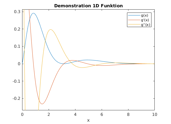
Grafik mit symbolischen Funktionen
clear, clf
syms x real
%assume(x,'real')
g(x) = (x+x*cos(x))/(2*exp(x)-log(x));      % Symb. Funktion

interval = [0,10];
ezplot(g ,interval); %fplot(g ,interval)

g1 = diff(g,x);                             % 1. Ableitung
hold on
ezplot(g1 ,interval); %fplot(g1 ,interval)

g2 = diff(g,2,x);                           % 2. Ableitung
ezplot(g2 ,interval); %fplot(g2 ,interval)

legend("g(x)","g'(x)","g''(x)") % Beschriftung der Plots
title("Demonstration 1D Funktion")
saveas(gcf,'g_1d.jpg')     % Speichere aktuelle Grafik in File
hold off
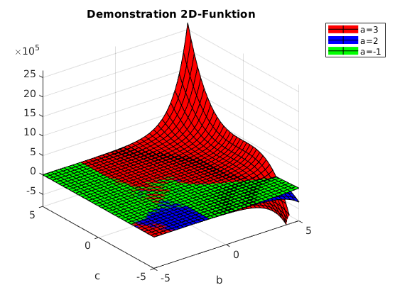
Visualisierung mit 2 Variablen (nur mit Funktion moeglich)
figure()           % 2. Grafikfenster
syms a b c;        % deklariere symbolische Variablen
f(a,b,c) = 3*(a-1)*(b^2+c^3)*(exp(a+b)-1)   % symbolische Funktion
% Präambel für Octave
if (exist('OCTAVE_VERSION', 'builtin') == 0)
    % Matlab branch
    fsurf( f(3,b,c));          % Flaeche g(b,c)

    % kombininierte Grafik fuer mehrere Werte von 'a'
    hold off                   % vorherige Grafik wird überschrieben
    fsurf( f(3,b,c),'r')       % Flaeche g_3(b,c) in 'red' (--> LineSpec)
    xlabel('b'); ylabel('c');  % Achsenbeschriftung
    hold on                    % fuege die naechsten Plots zur Grafik hinzu
    fsurf( f(2,b,c),'b');      % Flaeche g_2(b,c) in 'blue'
    fsurf( f(-1,b,c),'g');     % Flaeche g_1(b,c) in 'green'
    legend('a=3','a=2','a=-1') % Beschriftung der Plots
    title("Demonstration 2D-Funktion")
    saveas(gcf,'f_2d.jpg')     % Speichere aktuelle Grafik in File
    hold off                   % Grafik wird von nächstem Plot ueberschrieben
else
    % Octave branch
    ezsurf( f(3,b,c));          % Flaeche g(b,c)

    % kombininierte Grafik fuer mehrere Werte von 'a'
    hold off                   % vorherige Grafik wird überschrieben
    ezsurf( f(3,b,c))          % Flaeche g_3(b,c) in 'red' (--> LineSpec)
    xlabel('b'); ylabel('c');  % Achsenbeschriftung
    hold on                    % fuege die naechsten Plots zur Grafik hinzu
    ezsurf( f(2,b,c));         % Flaeche g_2(b,c) in 'blue'
    ezsurf( f(-1,b,c));        % Flaeche g_1(b,c) in 'green'
    legend('a=3','a=2','a=-1') % Beschriftung der Plots
    title("Demonstration 2D-Funktion")
    saveas(gcf,'f_2d.jpg')     % Speichere aktuelle Grafik in File
    hold off
end
f(a, b, c) =

(3*a - 3)*(b^2 + c^3)*(exp(a + b) - 1)
Publishing publish('v_1_a.m')