Ziege-Weide Aufgabe
Problemstellung und Loseung, siehe auch andere Loseungsmoeglichkeiten
Das symbolischen Paket von Matlab wird benutzt so weit es geht und zum Schluss muss numerisch geloest werden.
Contents
Variablen
symbolisch (gesuchte Groessen)
clc; clear all; %clf;

% syms l real positive;
l = sym('l','positive');          % Leinenlaenge
% syms x real positive;
x = sym('x','positive');          % x-wert des Schnittpunktes Wiesenkreis mit Leinenkreis
% gegebene Groessen, hier als Zahlenwert
R = 10;                           % Wiesenradius
assumeAlso(l<2*R);
Die beiden Kurven (symbolisch)
yR = R - sqrt(R^2-x^2);
yL = sqrt(l^2-x^2);
bestimme den Schnittpunkt
X = solve(yL - yR, x);

% Ausgabe
disp('Schnittpunkt der beiden Kurven')
pretty(yR); pretty(yL)
disp('ist')
pretty(X)
Schnittpunkt der beiden Kurven
                 2
10 - sqrt(100 - x )

      2    2
sqrt(l  - x )

ist
      /   (l - 20) (l + 20) \
l sqrt| - ----------------- |
      \          100        /
-----------------------------
              2
unbestimmtes Integrieren
I = int(yL - yR, x);
Einsetzen der Integrationsgrenzen
==> abgegraste Flaeche, symbolische Funktion A(l)
A = 2*int(yL - yR, x, 0,X);

% Ausgabe
disp('abgegraste Flaeche, Funktion A(l)')
pretty(A)
abgegraste Flaeche, Funktion A(l)
                    3
    / l #1 \       l  #1              2
asin| ---- | 100 + ----- - 10 l #1 + l
    \  20  /         40

                         /   4            \
                         |  l     2       |
                l #1 sqrt| --- - l  + 100 |
       / #1 \            \ 400            /
   asin| -- | + ---------------------------
       \  2 /                2

where

             /       2 \
             |      l  |
   #1 == sqrt| 4 - --- |
             \     100 /
Aufstellen der Gleichung, sodass die halbe Flaeche abgegrast wurde
Hier konvertieren wir eine symbolische Funktion in eine numerische Funktion.
Fs= A - pi*R^2/2;          % symbolische Funktion
F = matlabFunction(Fs);    % numerische Funktion

% Grafik
fplot(Fs,[0,2*R])
hold on
plot([0,2*R],[0 0 ],'b')
hold off
stringFs=strjoin(arrayfun(@char, Fs, 'uniform', 0));
title('Area = A(L)-pi*R^2/2'); xlabel('L')
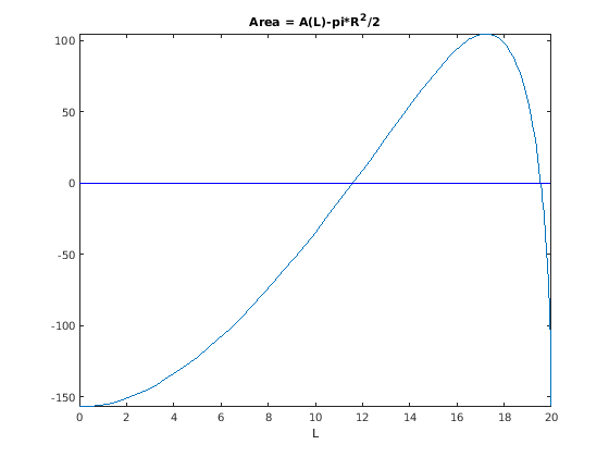
Bestimmen der Nullstelle (= Loesung) F(l)==0 mit Startlösung l=R
symbolisches (-> numerisches) Lösen von Fs(l)==0
L = solve(Fs,l)

% numerisches Lösen von F(l)==0 mit Startlösung l=R
L = fsolve(F,R)

%  Optimierungspaket: F(l)==0 mit Startlösung l=R
options = optimset('Display','iter');
L = fzero(F, R, options)                % only with optimization package
% options = optimoptions(@fsolve,'Display','iter') % Wie geht das genau?
% options = optimoptions(optimoptions(fsolve),'Display','iter')
Warning: Unable to solve symbolically. Returning a numeric solution using <a
href="matlab:web(fullfile(docroot, 'symbolic/vpasolve.html'))">vpasolve</a>.

L =

11.587284730181215178282335099335


Equation solved.

fsolve completed because the vector of function values is near zero
as measured by the value of the function tolerance, and
the problem appears regular as measured by the gradient.


L =

   11.5873


Search for an interval around 10 containing a sign change:
 Func-count    a          f(a)             b          f(b)        Procedure
    1              10      -34.2427            10      -34.2427   initial interval
    3         9.71716      -40.1279       10.2828      -28.2823   search
    5             9.6      -42.5422          10.4      -25.7928   search
    7         9.43431       -45.932       10.5657      -22.2528   search
    9             9.2      -50.6744          10.8      -17.2101   search
   11         8.86863      -57.2728       11.1314      -10.0123   search
   13             8.4      -66.3711          11.6      0.280816   search

Search for a zero in the interval [8.4, 11.6]:
 Func-count    x          f(x)             Procedure
   13            11.6      0.280816        initial
   14         11.5865    -0.0169335        interpolation
   15         11.5873  -2.35373e-06        interpolation
   16         11.5873   3.90799e-14        interpolation
   17         11.5873   3.90799e-14        interpolation

Zero found in the interval [8.4, 11.6]

L =

   11.5873
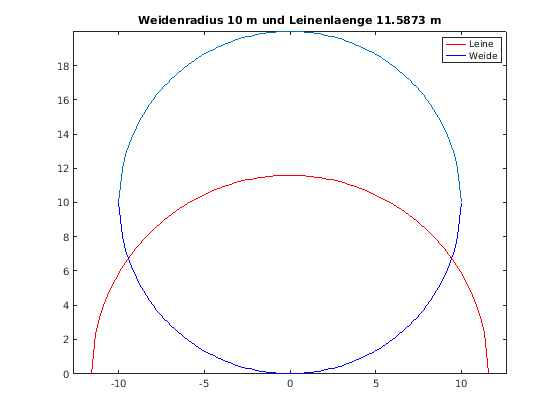
Grafik
n  = 100;
% Leinenkurve
xxL = linspace(-L, L, n);
yyL = subs(subs(yL,l,L),x,xxL);
% Wiesenkurve
xxR = linspace(-R, R, n);
yyR = subs(yR,xxR);

plot(xxL,yyL,'r');
hold on;
plot(xxR,yyR,'b');
plot(xxR,2*R-yyR);
plot(xxL,R);
axis equal
title(['Weidenradius ',num2str(R),' m und Leinenlaenge ',num2str(L),' m']);
legend('Leine','Weide');

% publish('ziege_wiese.m');