 |
 |
 |
| 50 percent noise | TV filtered | EFG filtered |
MEDICAL IMAGING PROJECTS
Edge-flat-grey scale image enhancement by convex functional minimization.
|
|
|
| 50 percent noise | TV filtered | EFG filtered |
These images are related to a baseline image constructed as follows. The baseline image is flat on a centered square where it assumes its maximum value, it is flat in the background where it assumes its minimum value, and otherwise it slopes linearly at the left between these two values. The left-most image shown is the baseline image plus 50 percent noise, i.e., the noise is normally distributed with zero mean and standard deviation equal to half the range of image values. The center image shown is the result of applying TV filtering to the noisy image; see [Rudin et al., 1992]. Note the classic staircasing in the region where the baseline image is linearly sloped. The right-most image shown is the result of applying an edge-flat-grey (EFG) filtering approach to the noisy image; see [Ito & Kunisch, 1999] and [Keeling, 2003]. Here, edge, flat, and grey scales, i.e., scales where the gradient is large, small, and intermediate, respectively, are clearly captured well.
The TV and EFG filters are defined in terms of minimizers for the functional:
for which the necessary optimality condition is expressed in the steady state for the following descent evolution equation:
(1)
This diffusion process can be further elucidated by the orthogonal decomposition:
(2)
where n denotes the derivative in the direction of grad u. Thus, with respect to level sets of u, the first term captures normal diffusion and the second captures tangential diffusion. Here, g(s) = f'(s)/s, and f''(s) is globally smooth and non-negative. Specifically:

(3)
For simplicity, suppose c = 1 and observe that the EFG penalty function takes the form on [0,1]:
(4)
Thus, the EFG penalty corresponds roughly to an Lp penalty on |grad u| where p varies as shown in the left plot following.

(5)
Also, shown on the right is a plot of f''(s) on the interval [0,1]. Note further that p(0) = p(1) = 1 and that f'''(s) is bounded. In light of Eqn. (3), the plot of f''(s) illustrates that diffusion normal to level sets of u is strictly positive for a range of gradient values, but drops to zero for sufficiently large and for vanishing gradients.
The numerical implementation of these filters involves discretization of the evolution equation in Eqn. (2). Specifically, the spatial discretization is built from Cartesian central differences among cells, where the nonlinear diffusivity g(|grad u|) is evaluated on cell interfaces. Also, for the TV filter, the function g(s) = 1/s is treated numerically as g(max{m,s}) for m equal to machine zero. The temporal discretization is achieved with implicit Euler time stepping, where the time stepping equations are solved with a Jacobi preconditioned conjugate gradient scheme. Full details and given in [Keeling, 2003].
Multiscale edge enhancement by nonlinear anisotropic diffusion.
 |
 |
 |
| highly blurred | PM filtered | BFB filtered |
The left-most image shown consists in a sum of six functions of the form a(1+bx2+cy2)-d chosen to create ever weaker edges while approaching the center of the image. The center image shown is the result of applying a routinely used Perona-Malik (PM) filter to the blurred image; see [Perona & Malik, 1987] and [Gerig et al., 1992]. Note that for the particular PM contrast parameter chosen here, the innermost edge is flattened, the next adjacent edge is sharpened, and other edges are essentially unaffected. The right-most image shown is the result of applying a balanced-forward-backward (BFB) diffusion filter to the blurred image; see [Keeling & Stollberger] for details. Here, all edges are sharpened equally well.
The PM and BFB filters are defined in terms of the nonlinear anisotropic diffusion equation:
where the diffusivities are given by:

(6)
Comparing the two evolution equations in Eqns. (2) and (6) reveals the variational connection with g(s) = f'(s)/s and:

(7)
Thus, the variational penalty function for PM is first convex and then concave, while for BFB it is globally concave. The diffusion decomposition in Eqn. (3) shows that both filters create forward diffusion tangent to level sets of u. However, for PM the diffusion normal to level sets is first forward and then backward. For BFB, not only is normal diffusion always backward, but its coefficient f'' has the same magnitude as that for the tangential diffusion g. This balance is the basis of the multiscale edge enhancement capability of the balanced-forward-backward diffusion filter.

(8)
The numerical implementation of these filters involves the discretization of the evolution equation shown in Eqn. (6). Specifically, the spatial discretization is built from diagonal central differences among cells, where the nonlinear diffusivity g(|grad u|) is evaluated at cell corners. Also, for the BFB filter, the function g(s) = 1/s2 is treated numerically as g(max{m,s}) for m equal to machine zero. For the PM filter, temporal discretization is accomplished with explicit Euler time stepping. For the BFB filter, temporal discretization is achieved with implicit Euler time stepping, where the time stepping equations are solved only approximately with a Jacobi preconditioned conjugate gradient scheme. Full details are given in [Keeling & Stollberger, 2000].
Application to contrast enhancement of medical images.
 |
 |
 |
| abdominal MRI | Gauss filtered | Gauss-TV filtered |
The left-most image shown is a moderately noisy MRI of the abdomen. The center image shown is the result of applying a routinely used Gauss filter to the MRI. Note the evident blur in the Gauss filtered image. The right-most image shown is the result of applying a Gauss-TV diffusion filter to the MRI. Here, there is a high contrast level along with a marked reduction in the noise level.
The Gauss filtered image was computed pixelwise merely by performing a weighted average of values in neighboring pixels from the MRI; see [Gonzalez & Woods]. On the other hand, the Gauss-TV filtered image was obtained using the diffusion approach in Eqn. (2) with the diffusivity:
which has roughly the same bell shape as that associated with Perona-Malik diffusivities:
(9)
However, here the diffusivity g(s) = 1 corresponds to Gaussian filtering in the sense that the image evolves according to the linear heat equation. Also, the diffusivity g(s) = c/s corresponds to TV filtering as seen earlier in the comparison with EFG filters. The combination of the Gaussian and TV filtering in Eqn. (9) gives:
Therefore, because of Eqn. (3), diffusion normal to level sets is never backward as seen with the edge enhancing filters. As a result, the diffusivity in Eqn. (9) is edge-preserving for edges with |grad u| > c. Also, it is isotropically dissipative for noise with |grad u| < c.

(10)
In terms of EFG filters, the Gauss-TV filter treats images as consisting of two scales: edge and grey. This combination is quite effective for contrast enhancement of medical images, and can be particularly useful to increase lesion conspicuity for example. On the other hand, the additional treatment of flat scales with EFG filters has been found to excessively flatten small slope regions in these images. Specifically, this flattening effect causes a loss of a natural three dimensional appearance. On the other hand, the flattening resulting from EFG, PM, and BFB filters can be used to advantage as a preprocessor for a segmentation procedure. For further details, see [Keeling, 2003].
Application to magnetic resonance diffusion tensor imaging.
 |
 |
 |
| FA brain map | Gauss filtered | Gauss-TV filtered |
Magnetic resonance diffusion tensor imaging is a procedure used for mapping the diffusion properties of water in tissues; see [Bammer, Augustin et al., 2000]. Such diffusion is considerably anisotropic and is influenced by the underlying tissue organization and damage thereto. As a result, this imaging technique has naturally advanced into everyday routine clinical applications. The work shown here is aimed at the contrast enhancement and noise reduction in such images, using the Gauss-TV approach outlined above.
The water diffusion properties of interest can be detailed as follows. The flux of water molecules is described locally by J = -D grad C, where grad C is a concentration gradient driving the diffusion, and D is the diffusion tensor relating the gradient vector to the resulting flux vector according to the properties of the underlying diffusion medium. The diffusion tensor is measured using magnetic resonance as follows. First, when a magnetic field pulse with magnitude gradient G(t) is added to the baseline pulse sequence, which would otherwise lead to the measured image M0, a diffusion-weighted image M is measured satisfying:
Here, g is the gyromagnetic ratio of hydrogen, the element in water upon which MRI keys. Also, the gradient pulse G(t) occurs during the pulse sequence interval [0,TE] where TE is the echo time measured in milliseconds. See [Hornak, 1996] for details. Now, because of the symmetry in D, there are seven independent pointwise unknowns among M0 and D. Therefore, using seven linearly independent gradient fields in successive pulse sequences provides sufficient diffusion-weighted images to permit the diffusion tensor to be determined pointwise.

(11)
In particular, imaging the rotational invariants of D has been used to advantage for diagnostic purposes. For instance, the trace of D provides an orientationally averaged apparent diffusivity:
and is used to increase lesion conspicuity by suppressing nearby anisotropic effects. On the other hand, when anisotropic effects are of primary concern, as in the evaluation of nerve fiber tracts, the fractional anisotropy (FA) can be imaged:
(12)
It is this fractional anisotropy which is mapped in the three images appearing above.
(13)
The left-most image shown above is a noisy FA map of the brain, obtained using unfiltered diffusion-weighted images, from which the diffusion tensor images were derived and used in Eqn. (13). The next two images are the results of using the filters discussed in detail earlier for the abdominal MRI. Specifically, the center image shown is the result of applying the Gauss filter to the diffusion tensor images before computing the FA map. As before, note the evident blur in the Gauss filtered image. The right-most image shown is the result of applying the Gauss-TV diffusion filter to the diffusion tensor images before computing the FA map. Again, there is a high contrast level along with a marked reduction in the noise level. See [Keeling, Bammer, Fazekas & Stollberger, 2000].
Restoration of images corrupted by noise and background variations.
 |
 |
| nonuniform background | uniform background |
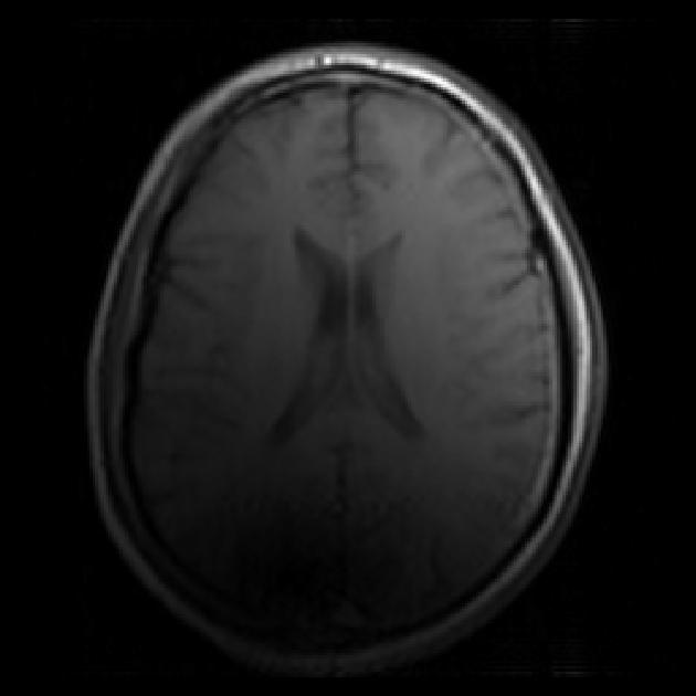
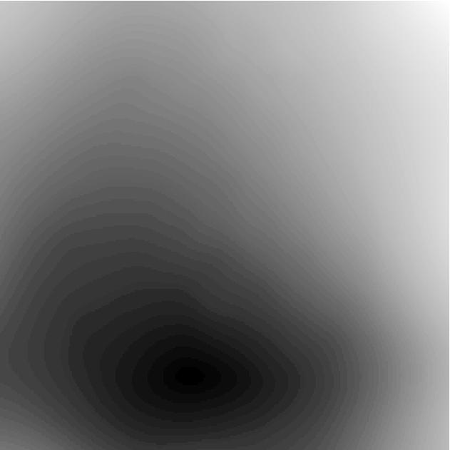
The purpose of this project is to investigate the enhancement of magnetic resonance images in which broad-band clinical information coexists not only with high gradient noise but also with a slowly varying background variation often seen in MR images. Specifically, this background variation occurs because of the difficulty in generating an ideal, uniform magnetic field for the production of an MR image; see [Hornak, 1996]. For instance, the left image shown above is an MRI of the pelvis. Here, the wide field of view frustrates the task of creating a uniform magnetic field over the entire image region. As a result, the nonuniform background is manifested with the image intensity much higher near the center than toward the periphery. On the other hand, the right image shown is an MRI obtained from an in vitro arthrosclerotic vessel. Here, the field of view is much narrower and there is less difficulty with generating a uniform magnetic field over the sample.
An accepted model for this background variation involves approximating a measured intensity u~ with a product mu where m > 0 is a smooth multiplier field adjusting for the nonhomogeneous magnetic field strength so that u corresponds to the intensity that would be measured in a uniform magnetic field; see [Pham & Prince, 1998]. In fact, the objective is to determine m and u, where u~/m is free of the background variation appearing in u~, and u is free of the noise still present in u~/m.
To achieve this objective, the pair (m,u) is determined as a minimizer for the functional:
Here, f is a convex function, as in Eqn. (9), used to penalize noisy oscillations in u without smoothing intensity discontinuities at tissue boundaries. The remaining penalty terms control the noisy oscillations and the curvature accumulations in m, depending upon regularization parameters a > 0 and b > 0, respectively. The optimality system for J(m,u) has been derived and novel numerical techniques have been formulated for the determination of m and u. For further details, see [Keeling & Bammer, 2004] and [Keeling & Haase, 2007].

(14)
Phase unwrapping by regularized phase construction in a region growing setting.
 |
 |
| wrapped noisy phase | unwrapped noisy phase |
The raw data measured for an MR image are understood in terms of both a magnitude and a phase of a complex signal on the basis of the following model; see [Hornak, 1996]. To create the MR signal, a uniform magnetic field is first applied to align the magnetization of the hydogen proton spins in the body. Then, a sufficient secondary magnetic field pulse is applied to excite the protons at a resonant frequency so that the local net magnetization is pushed away from the alignment axis and into the orthogonal plane as it begins to precess about the axis at the resonant frequency. The magnetization precessing in this plane is modeled as a complex magnetization, with real and imaginary parts corresponding to projections onto orthogonal axes therein. The magnitude of this complex magnetization is related to the local hydrogen density, the property normally imaged with MRI. On the other hand, the phase of the magnetization can be related to local conditions which alter the local resonant frequency of hydrogen protons. For instance, the hydrogen protons in water have a slightly different resonant frequency than the hydrogen protons in fat.
However, given a noisy complex magnetization m~ = r~exp(ip~), determining the underlying phase p~ is nontrivial; see [Song, 1995] and [Liang, 1996]. For instance, the derived phase tan-1(Im{m~}/Re{m~}) is necessarily wrapped into the range (-Pi/2,Pi/2]. As a result, phase jumps of Pi can appear as seen in the wrapped phase image shown above on the left but not in the unwrapped phase image on the right. This phase map arises in the course of using the Dixon method to distinguish fat and water around the knee; see [Flevaris, 2000]. A detailed examination of these images shows that the presence of image noise can frustrate the computation of an accurately unwrapped phase. Furthermore, steep gradients in the phase must evidently be allowed at tissue boundaries. Therefore, it is required not only to avoid phase wrappings but also to avoid smoothing natural discontinuities while removing noise to obtain an appropriately filtered phase p ~= p~.
It is proposed that the objectives can be achieved with the following natural variational approach:
Here, r is an estimate of the signal magnitude. Also, f1 and f2 are convex functions, as in Eqn. (9), designed to penalize oscillations in r and p while allowing them to exhibit natural discontinuities. Preliminary computations on model problems demonstrate that this variational approach can be performed in a region-growing fashion to achieve highly accurate phase distributions.

(15)
Well-posedness analysis of new image enhancement schemes.
This area of research is aimed most immediately at establishing well-posedness results for the diffusion filters in Eqns. (2) and (6), where the diffusivity is unbounded. For example, Eqns. (4) and (7) show that the TV, EFG, and BFB diffusivities are unbounded for vanishingly small gradients. As stated earlier, such an unbounded diffusivity g(s) is treated numerically as g(max{m,s}) where m is equal to machine zero. Nevertheless, computational findings demonstrate that results are insensitive to variations in a sufficiently small m. This observation suggests the following continuous dependence property.
First, let U(t) in RN be a vector of pixel values approximating u(t) in the diffusion equation on any interval [0,T]. Then, suppose the matrix-vector product G(U)U is a spatial discretization of the nonlinear diffusion as described earlier. Also, let Gm(U)U denote the corresponding discretization with g(s) regularized by g(max{m,s}). Then, the well-posedness properties for the semi-discrete problem:
are well understood [Weickert, 1998]. For a fixed m > 0, let the solution be denoted by Um in C1([0,T],RN). Then, the computational results suggest that the functions {Um} converge to a function U* in C0([0,T],RN) as m -> 0.

(16)
Observations about the desired continuous dependence property include the following. First, an m independent C1 bound on the solutions to Eqn. (16) provide subsequential convergence in C0 by compactness. The challenge is to obtain a unique characterization of subsequential limits. Studies of the fixed points of:
show that there exist examples where, for m = 0, it is possible that this equation can only be solved nonuniquely by discontinuous functions. However, the corresponding limit of fixed points as m -> 0 is unique and continuous. Thus, the characterization of U* must not involve equations of the form Eqn. (16) or (17).
(17)
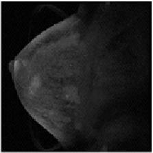
Image registration by optical flow with maximal rigidity.
 |
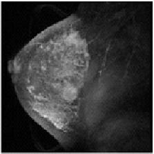 |
| breast MR at t1 | breast MR at t2 |
The diagnostic use of medical image sets in a clinical setting implicitly requires a point by point correspondence between the same tissue sites in separate images. For example, the two images shown above were taken before and after the injection of a contrast agent during a mammography examination. To monitor the uptake of the contrast agent at specific, potentially pathological sites, it is necessary to track the site of interest through the tissue motion occuring during the examination. Thus, what is needed finally is an explicit coordinate transformation that will map any point in one image to its corresponding point in the other. With such a mapping, images are said to be registered. See [Thirion, 1998] and [Rueckert et al., 1999].
In this work, two given images I0, I1: P (in RN) -> R are registered by morphing one to the other according to an appropriate variational principle. This morphing process is defined by two components. First, is an optical flow f(x,t): P x [0,1] -> P determined from an optical flow field F(y,t): P x [0,1] -> RN according to:
Second, is a family of images I(x,t): P x [0,1] -> R related ideally to the optical flow field F by:

(18)
Here, t is a pseudo-temporal variable used to parametrize the morph components. Thus, as t passes from 0 to 1, a point x0 in the image I0 at time t = 0 is transported by the optical flow to the point x1 = f(x0,1) in the image I1 at time t = 1. Also, the morphed images are given by I(f(x,t),t).

(19)
The registration given by (I,F) is determined by minimizing the functional:
where n denotes the outwardly directed unit normal vector at S, the boundary of P. The first term here penalizes the convection equation in Eqn. (19) and thus minimizes intensity variations along optical flow trajectories. The second term penalizes the departure of the optical flow field gradient from skew symmetry and thereby maximizes the rigidity of the displacements resulting from the optical flow. This term can also be viewed as a penalty on the elastic energy stored in the displacements corresponding to the coordinate transformations. It is proposed here that such a selection criterion for the optical flow is well suited for medical registration since human tissue is more elastic than it is fluid and other standard penalty terms give rise to unnaturally aqueous effects. The final penalty term is used so that detailed features in the given images are preserved in the morphed images as sharply as possible. The convex functions f1 and f2 are chosen, as in Eqn. (9), to penalize noisy oscillations without smoothing intensity discontinuities at tissue boundaries. The optimality system for J(I,F) has been derived and novel numerical techniques have been formulated for the determination of I, F, and f. For further details, see [Keeling & Ring, 2005].

(20)
Kernel estimation, for
perfusion imaging, and
tracer exchange kinetics imaging,
by discontinuity-preserving spatio-temporal regularization.
Pathophysiological properties of breast tumors are evaluated clinically from an examination in which the tumor is imaged repeatedly to measure the uptake of an injected contrast agent. The amount of injected tracer and the amount of absorbed tracer are related by a convolution whose kernel provides the desired diagnostic information. Specifically, let Ca(t) be the tracer concentration at time t in an artery feeding the tumor. Also, let Cr(x,t) be the tracer concentration at tissue site x at time t. Assume that both Ca(t) and Cr(x,t) can be measured by imaging the feeding artery and the tumor respectively. Then these concentrations are related according to:
Here, the nature of the kernel R(x,t) can be understood by considering an impulsive injection Ca(t) = delta(t). In this case, Cr(x,t) = R(x,t) is the concentration of tracer remaining at the tissue site x after the impulsive injection; therefore, R(x,t) is a non-increasing function of t. In fact, the maximal temporal decay rate of R, or other temporal shape parameters, can be imaged spatially to provide the required diagnostic information.
(21)
Note that the measurement Cr(x,t) suffers from a low signal-to-noise ratio because of the temporal resolution required. As a result, it is inappropriate to decouple the spatial and temporal variations in Eqn. (21). Rather than to filter Cr spatially for determining R, it is proposed to solve the inverse problem directly for R by using unfiltered data and imposing spatio-temporal regularity constraints on R. This spatio-temporal regularization must first filter the effect of measurement noise while allowing discontinuities which may occur. Such discontinuities can occur spatially at tissue boundaries, and they can occur temporally in case of poor perfusion and a resulting plug flow. Further, the temporal regularization must involve explicit monotonicity constraints, as opposed to implicit ones seen for example in [Ostergaard et al., 1996]. Thus, it is proposed to solve Eqn. (21), written in operator form as Cr = KaR, by minimizing the functional:
subject to: R(x,t) non-increasing at each x in P. Here, P is the tumor region, [0,T] is the measurement period, Grad is the gradient in P x [0,T], and f is a convex function, as in Eqn. (9), designed to penalize noisy oscillations in R while permitting the occurrence of natural discontinuities. The optimality system for J(R) has been derived and novel numerical techniques have been formulated for the determination of R. For further details, see [Keeling, Kogler & Stollberger, 2009] and [Keeling, Bammer & Stollberger, 2007].
(22)
Coil sensitivity estimation for high-speed parallel magnetic resonance imaging strategies.
 |
 |
| sensitivity weighted | coil sensitivity |
The continuing development of magnetic resonance imaging has driven the need for increased image acquisition speed, for instance, to increase temporal resolution. Sensitivity encoding (SENSE) is a technique for reducing the scan time by employing multiple receiver coils which measure the magnetic signal in parallel at a reduced sampling rate; see [Bammer, Stollberger et al., 2000]. The sampling rate is reduced by a factor corresponding to the number of coils. Also, since the reduced sampling rate is below that required to capture the full information content in the signal, each measurement is aliased.
Specifically, suppose the sampling rate is only reduced in the phase-encoding direction, which corresponds to the vertical or say y direction in the image after Fourier transforming the signal; see [Hornak, 1996] for details. Suppose there are N coils each sampling in the phase-encode direction at a rate reduced by a factor of N. Now let Mi be the image that would be measured by the ith coil with full sampling, and let Mi be the image measured with reduced sampling. If the vertical dimension of the image Mi is Y, then Dy = Y/N is the vertical dimension of the image Mi. If both images are continued by periodicity, then the aliasing in Mi implies:
It is desired to decode this aliasing and to use the rapidly obtained images {Mi: i = 1,...,N} to construct the underlying image M which would be measured less rapidly in the usual manner. For this, note that Mi = Ci M where Ci is the coil sensitivity for the ith coil. Given the coil sensitivities, the following equations determine the desired image M:

(23)
Separate measurements can be made to determine a coil sensitivity. Suppose there is a body coil with which a homogeneous signal Mbody can be measured. Also, let Msurf be the nonhomogeneous signal measured simultaneously by a surface coil. Then the coil sensitivity is determined from the quotient:
(24)
For example, the left image shown above depicts CMbody = Msurf for a given coil sensitivity C shown in the right image. Evidently, the quotient becomes indeterminant in regions of low signal. Also, the regions of strong signal can be spatially discontinuous because of sudden changes in tissue properties. On the other hand, the coil sensitivity is a globally smooth distribution. Thus, the objective is to reconstruct the coil sensitivity to satisfy Eqn. (25) as nearly as possible while filtering the quotient appropriately to preserve its known regularity.

(25)
To achieve the objective, C is determined as a minimizer for the following cost:
Here, a and b are positive weights for penalty terms respectively controlling the noisy oscillations and the curvature accumulations in C. Furthermore, these parameters control the trade-off between their regularizations and the reduction of the residual |CMbody - Msurf|. The optimality system for J(C) has been derived and novel numerical techniques have been formulated for the determination of C. For further details, see [Keeling & Bammer, 2004] and [Keeling & Haase, 2007]

(26)
References.