Contents

CompMath-Vorlesung 4.11.2022

Wiederholung Kurve in der Ebene Kurven, Flaechen im Raum

close all; clear; clc

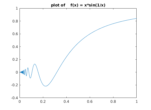
Plot einer Funktion y:=f(x) = x*sin(1/x) im Intervall [0.001,1]

x = linspace(0.001,1,1001);
y = x.*sin(1./x);
plot(x,y)                                  % numerische Funktion via Polygonzug
title('plot of    f(x) = x*sin(1/x)')

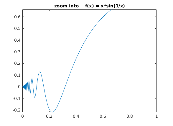
Alternativ

fplot(@(x) x*sin(1/x),[0.001,1])           % numerische Funktion, wie oben
title('zoom into    f(x) = x*sin(1/x)')

Warning: Function behaves unexpectedly on array inputs. To improve performance,
properly vectorize your function to return an output with the same size and
shape as the input arguments. 

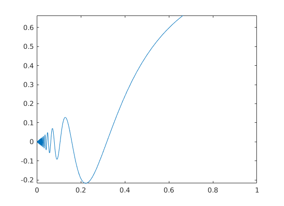
Alternativ

fplot('x*sin(1/x)',[0.001,1])             % symbolische Funktion, wie oben
% ezplot('x*sin(1/x)',[0.001,1])          % octave

Warning: fplot will not accept character vector or string inputs in a future
release. Use fplot(@(x)x.*sin(1./x)) instead. 

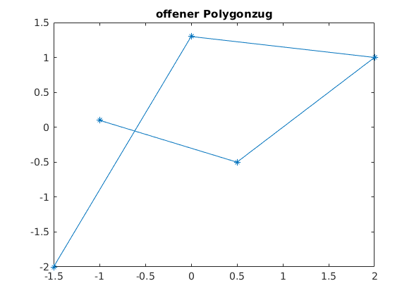
Zeichnen eines Polgonzuges

xy = [  -1,  0.5, 2 ,   0, -1.5;            % x-coords
       0.1, -0.5, 1 , 1.3, -2   ];          % y-coords

plot(xy(1,:),xy(2,:),'*-')
title('offener Polygonzug')

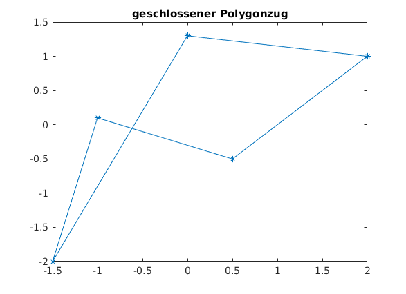
geschlossener Polygonzug

xy_g = [xy xy(:,1)]
plot(xy_g(1,:),xy_g(2,:),'*-')
title('geschlossener Polygonzug')

xy_g =

   -1.0000    0.5000    2.0000         0   -1.5000   -1.0000
    0.1000   -0.5000    1.0000    1.3000   -2.0000    0.1000

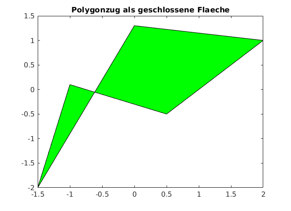
Alternativ mit originalen Koordinaten

fill(xy(1,:),xy(2,:),'g')
title('Polygonzug als geschlossene Flaeche')

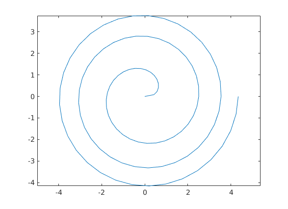
Parametrisierte Kurve in 2D

clear, clc, clf
t = linspace(0,6*pi,100);
x = sqrt(t).*cos(t);
y = sqrt(t).*sin(t);
plot(x,y)
axis equal

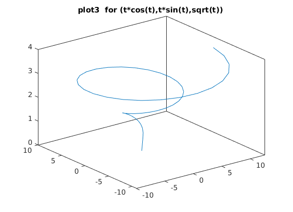
Parametrisierte Kurve im Raum (ezplot3, plot3)

siehe Kernbichlerskript Sect.15

wir plotten x(t) = t*cos(t); y(t) = t*sin(t); z(t) = sqrt(t)

via ezplot3

clear, clc, clf
ezplot3('t*cos(t)','t*sin(t)','sqrt(t)',[0,4*pi])
box on

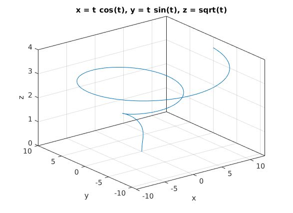
via plot3

clc; clf
t = linspace(0,4*pi,51);
x = t.*cos(t);
y = t.*sin(t);
z = sqrt(t);
plot3(x,y,z)
box on
title('plot3  for (t*cos(t),t*sin(t),sqrt(t)) ')

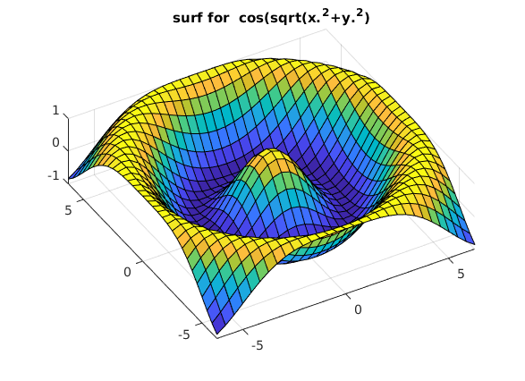
Flaeche im Raum (surf)

Zeichnen von z(x,y)

clear, clc, clf
x = linspace(-2*pi,2*pi,31); % 1D Koord. erzeugen
y = x;

[XX,YY] = meshgrid(x,y);     % Gitter erzeugen

ZZ = cos(sqrt(XX.^2+YY.^2)); % z(x,y)
surf(XX,YY,ZZ)
title('surf for  cos(sqrt(x.^2+y.^2)')
view([-30,70])               % Grafik in "gute" Position drehen

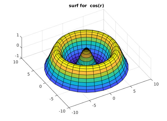
Flaeche im Raum (Polar+surf)

Zeichnen von z(r) = cos(r) = cos(sqrt(x*x+y*y))

clear, clc, clf
phi = linspace(0,2*pi,31); % 1D Koord. erzeugen
% r = linspace(0,15,31);
r = linspace(0,sqrt(2)*2*pi,31);

[PP,RR] = meshgrid(phi,r);  % Meshgrid mit Polarkoord.

ZZ = cos(RR); % z(r)
% ZZ = cos(RR).*PP/6;

[XX,YY] = pol2cart(PP,RR);  % Meshgrid mit kart. Ksoord.

surf(XX,YY,ZZ)
title('surf for  cos(r)')
view([-30,70])               % Grafik in "gute" Position drehen

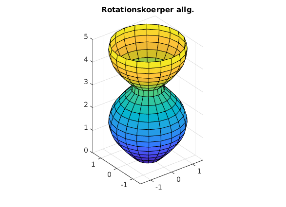
Rotationskoerper (via Cylinder) mit radius = f(hoehe)

clear, clc, clf
H = 5; % Hoehe
z = linspace(0,H,21);   % Hoehe (z) diskretisieren
r = abs(sin(z))+0.5;    % radius(z) is eine Funktion der Hoehe

[XX,YY,ZZ] = cylinder(r);
%  ZZ aus cylinder ist stets aus [0,1]
ZZ = ZZ*(H-0)+0;                  % Hoehe korrekt behandeln
surf(XX,YY,ZZ);
title('Rotationskoerper allg.')
axis equal

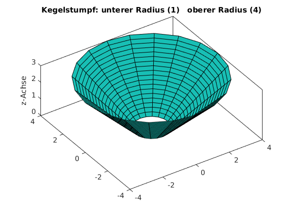
Kegelstumpf (via Cylinder)

clear, clc, clf
hoehe  = 3;
n = 20;
low_r  = 1; % unterer Radius
high_r = 4; % oberer Radius

r = (high_r-low_r)/hoehe*linspace(0,hoehe,n-1)+low_r;
[XX,YY,ZZ] = cylinder(r);  % Achtung !!  z aus [0,1]
ZZ = hoehe*ZZ;             % z korrekt skalieren
surf(XX,YY,ZZ,ones(size(ZZ)))
view([-34,34])
axis equal
grid off
box on
zlabel('z-Achse')
title(['Kegelstumpf: unterer Radius (',num2str(low_r),')   oberer Radius (',num2str(high_r),')'])

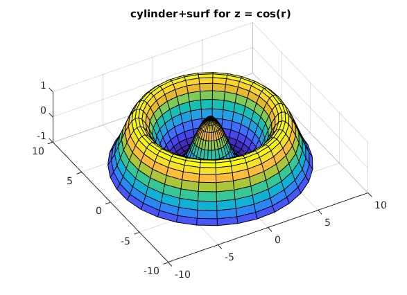
Rotationskoerper mit hoehe = f(radius)

(unsere Funktion z(r) = cos(r) nochmals betrachtet)

clear, clc, clf
r = linspace(0,sqrt(2)*2*pi,31);
[XX,YY,RR] = cylinder(r,31);
% Jetzt berechnen wir die Hoehe aus dem Radius
RR=(max(r)-min(r))*RR+min(r);
ZZ=cos(RR);         % Achtung, jetzt ist zz = zz(rr)
surf(XX,YY,ZZ)
title('cylinder+surf for z = cos(r)')
view([-30,70])               % Grafik in "gute" Position drehen

You have publish manually from the command window in case of figures

see MATLAB answers.

publish('v_5_b.m');

MathWorks

Published with MATLAB® R2019a