Contents

CompMath-Vorlesung 4.11.2022

Kurven; Flaechen, Koerper im Raum

close all; clear; clc

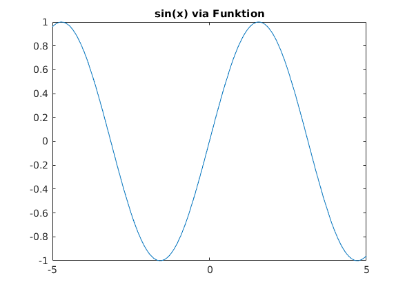
Kurve in 2D via Funktion

Graph von sin(x) mit x aus [-5,5]

fplot(@(x) sin(x),[-5,5])
title('sin(x) via Funktion')

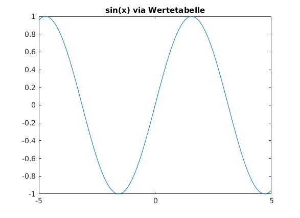
Kurve in 2D via Wertetabelle

x = linspace(-5,5,101);
y = sin(x);
plot(x,y)
title('sin(x) via Wertetabelle')

% see also: comet, semilogx, semilogy, loglog, plotyy, fill

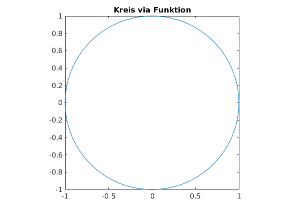
parametrisierte Kurve in 2D via Funktion

Beispiel Kreis via Funktion

fplot(@(phi) cos(phi), @(phi) sin(phi), [0,2*pi])
axis equal
title('Kreis via Funktion')

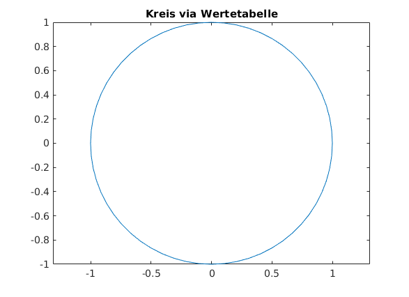
parametrisierte Kurve in 2D via Wertetabelle

phi = linspace(0,2*pi,61);         % Parameter
x = cos(phi);                      % x(phi)
y = sin(phi);                      % y(phi)
plot(x,y)
axis equal
title('Kreis via Wertetabelle')

% see also: polarplot, pol2cart, cart2pol

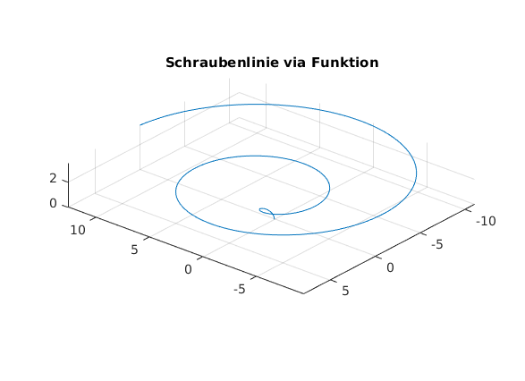
Parametrisierte Kurve in 3D via Funktion

eine Schraubenlinie via Funktion

fplot3(@(t) t.*cos(t), @(t) t.*sin(t),  @(t) sqrt(t), [0,4*pi])
view([-140,26])
axis equal
title('Schraubenlinie via Funktion')

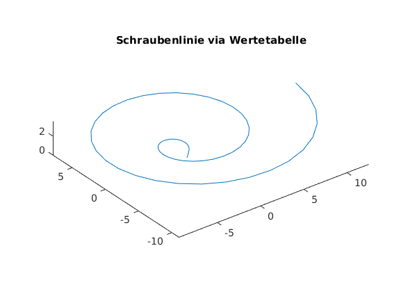
Parametrisierte Kurve in 3D via Wertetabelle

t = linspace(0,4*pi,61);         % Parameter
x = t.*cos(t);                   % x(t)
y = t.*sin(t);                   % y(t)
z = sqrt(t);                     % z(t)
plot3(x,y,z)
axis equal
title('Schraubenlinie via Wertetabelle')

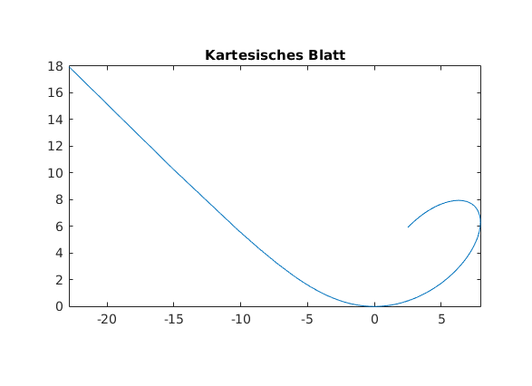
Beispiel kartesisches Blatt

Wiki

a = 5;
fplot(@(t) 3*a*t./(1+t.^3), @(t) 3*a*t.^2./(1+t.^3), [-pi/4,3*pi/4])
axis equal
title('Kartesisches Blatt')

% see also: comet3, fill3

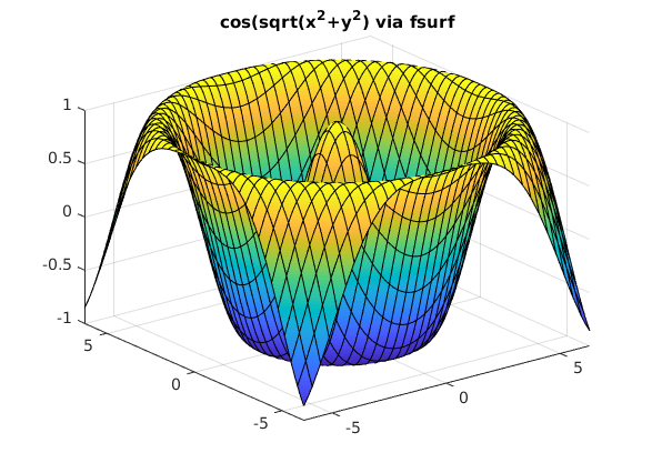
Flaeche im Raum (fsurf, kartesische Koord.)

% z(x,y) = cos(sqrt(x^2+y^2))
clear, clc, clf
fsurf(@(x,y) cos(sqrt(x.^2+y.^2)), [-2*pi,2*pi])
title('cos(sqrt(x^2+y^2) via fsurf')

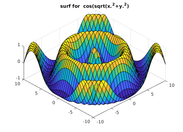
Flaeche im Raum (surf, kartesische Koord.)

clear, clc, clf
%
x = linspace(-10,10,31); y = linspace(-10,10,41);
%
[XX,YY] = meshgrid(x,y);         % logisches Rechteckgitter (Tensorprodukt)
ZZ = cos(sqrt(XX.^2+YY.^2));

surf(XX,YY,ZZ)
title('surf for  cos(sqrt(x.^2+y.^2)')
view([-44,58]);
% snapnow

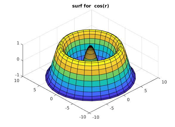
dieselbe Flaeche im Raum (surf, Polarkoordinaten)

Zeichnen von z(x,y) = z(phi,r)

clear, clc, clf
%
phi = linspace(0,2*pi,31); % 1D Koord. erzeugen
r = linspace(0,3*pi,31);

[PP,RR] = meshgrid(phi,r); % Gitter erzeugen
ZZ = cos(RR);              % z(phi,r)  wie oben
%ZZ = cos(RR)./(RR+1);     % interessantere Fkt.

[XX,YY,ZZ] = pol2cart(PP,RR,ZZ); % Konvertiere in kartesische Koord.
surf(XX,YY,ZZ);
title('surf for  cos(r)')
view([-44,58]);

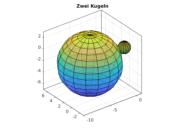
Kugel (sphere + surf)

clear, clc, clf
% Kugel in Mittelpunktslage mit Radius 1
[XX,YY,ZZ] = sphere(16);  % Gitter der Kugeloberflaeche
surf(XX,YY,ZZ)
hold on
% Kugel mit Radius R und Mittelpunkt MP
R = 5;
MP = [-5,2,-2];
XX = XX*R + MP(1); YY = YY*R+MP(2); ZZ = ZZ.*R+MP(3);

surf(XX,YY,ZZ)
box on
axis equal
alpha(0.7);              % Transparenz
title('Zwei Kugeln')

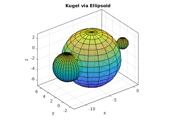
und Kugel als Ellipsoid (x-Koord. des Mittelpunktes nochmals verschoben)

[XX,YY,ZZ] = ellipsoid(MP(1)-5,MP(2),MP(3),R/2,R/2,R/2,32);
surf(XX,YY,ZZ);
box on
axis equal
xlabel('x'),ylabel('y'), zlabel('z')
title('Kugel via Ellipsoid')

% %% von Kugel ausgehend ein Flaeche radius(phi,theta) zeichnen
% clear, clc, clf
% [XX,YY,ZZ] = sphere(37);
% [PP,TT,RR] = cart2sph(XX,YY,ZZ)     % kartesisch --> polar
% RR = RR.*(1.5+cos(2*PP));           % Radiusfunktion
% [XX,YY,ZZ] = sph2cart(PP,TT,RR);    % polar --> kartesisch
% surf(XX,YY,ZZ);
% title('von Kugel ausgehend ein Flaeche radius(phi,theta) zeichnen')
% axis equal

% %%  Kugel: Radius mit Zufallsdaten
% clear, clc, clf
% [XX,YY,ZZ] = sphere(37);
% [PP,TT,RR] = cart2sph(XX,YY,ZZ)     % kartesisch --> polar
% RR = RR.*(1+rand(size(RR))*0.15);   % Radius mit Zufallsdaten
% [XX,YY,ZZ] = sph2cart(PP,TT,RR);    % polar --> kartesisch
% surf(XX,YY,ZZ);
% title('Kugel: Radius mit Zufallsdaten')
% axis equal

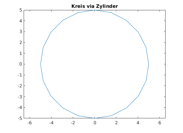
Kreis via cylinder

clear, clc, clf
n = 31;       % Anzahl der Punkte zur Darstellung
Radius = 5;
[XX,YY,ZZ] = cylinder(Radius);
x = XX(1,:); y = YY(1,:);    % Kreis mit Mittelpunk (0,0)
clear XX YY ZZ               % nicht mehr benoetigte Matrizen
plot(x,y)
axis equal

title('Kreis via Zylinder')

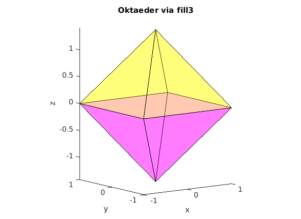
Oberflache eines Oktaeders via Einzelflaechen und fill3

clear, clc, clf
% Eckpunkte zeilenweise

P = [  1  1  0 ; ...
      -1  1  0 ; ...
      -1 -1  0 ; ...
       1 -1  0 ; ...
       0  0  sqrt(2); ...
       0  0 -sqrt(2) ]
%
idx = [1 2 5]  ;                         % Indexvektor: Welche Punkte?
fill3( P(idx,1), P(idx,2), P(idx,3), 'y' );
hold on
idx = [2 3 5]  ;                         % Indexvektor: Welche Punkte?
fill3( P(idx,1), P(idx,2), P(idx,3), 'y' );
%
idx = [3 4 5] ;
fill3( P(idx,1), P(idx,2), P(idx,3), 'y' );
%
idx = [4 1 5];
fill3( P(idx,1), P(idx,2), P(idx,3), 'y' );
%
idx = [1 2 6] ;                          % Indexvektor: Welche Punkte?
fill3( P(idx,1), P(idx,2), P(idx,3), 'm' );
%
idx = [2 3 6];                           % Indexvektor: Welche Punkte?
fill3( P(idx,1), P(idx,2), P(idx,3), 'm' );
%
idx = [3 4 6];
fill3( P(idx,1), P(idx,2), P(idx,3), 'm' );
%
idx = [4 1 6];
fill3( P(idx,1), P(idx,2), P(idx,3), 'm' );

alpha(0.3);          % Mass der Undurchsichtigkeit aus [0,1]
axis equal

idx = [1 2 3 4];  % Mittelebene
%fill3( P(idx,1), P(idx,2), P(idx,3), 'r' );
xlabel('x'); ylabel('y'); zlabel('z')
title('Oktaeder via fill3')
view([-36,10])

P =

    1.0000    1.0000         0
   -1.0000    1.0000         0
   -1.0000   -1.0000         0
    1.0000   -1.0000         0
         0         0    1.4142
         0         0   -1.4142

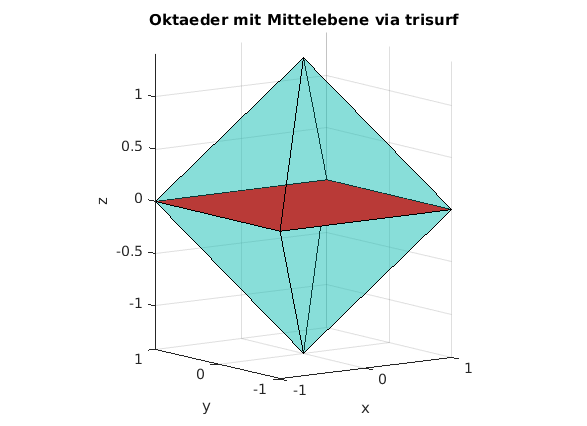
Oberflache eines Oktaeders via trisurf

clear, clc, clf
% Eckpunkte zeilenweise
verts = [  1  1  0 ; ...
          -1  1  0 ; ...
          -1 -1  0 ; ...
           1 -1  0 ; ...
           0  0  sqrt(2); ...
           0  0 -sqrt(2) ]

% Beschreibung der Teildreiecke (connectivity matrix)
%
faces = [ 1 2 5 ; ...
          2 3 5 ; ...
          3 4 5 ; ...
          4 1 5 ; ...
          1 2 6 ; ...
          2 3 6 ; ...
          3 4 6 ; ...
          4 1 6 ]

trisurf(faces, verts(:,1), verts(:,2), verts(:,3) )

alpha(0.3);          % Mass der Undurchsichtigkeit aus [0,1]
axis equal

% und nun noch die Mittelebene einzeichnen
hold on
idx = [1 2 3 4];  % Indizes der Eckpunkte
fill3( verts(idx,1), verts(idx,2), verts(idx,3), 'r' );
xlabel('x'); ylabel('y'); zlabel('z')
title('Oktaeder mit Mittelebene via trisurf')
view([-36,10])

verts =

    1.0000    1.0000         0
   -1.0000    1.0000         0
   -1.0000   -1.0000         0
    1.0000   -1.0000         0
         0         0    1.4142
         0         0   -1.4142


faces =

     1     2     5
     2     3     5
     3     4     5
     4     1     5
     1     2     6
     2     3     6
     3     4     6
     4     1     6

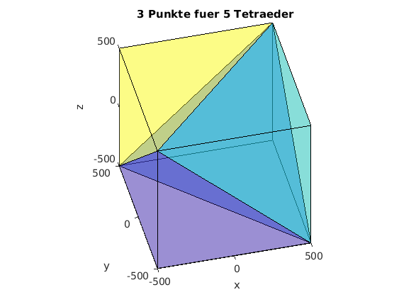
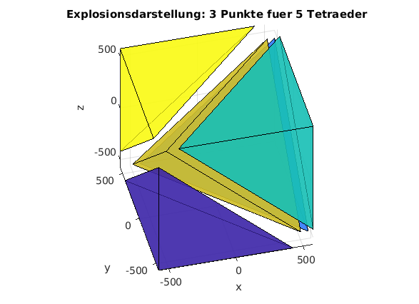
Wuerfel in 5 Tetraeder zerlegt

clear, clc, clf
% Koordinaten der Eckpunkte
KK = [-500 -500 -500;...
       500 -500 -500;...
      -500 500 -500;...
       500 500 -500;...
      -500 -500 500;...
       500 -500 500;...
       -500 500 500;...
       500 500 500];

%  Zuordnung der Eckpunkte zu den Tetraedern (C-Indexing)
Tets = [ 0 1 2 4; 2 1 3 7; 1 4 5 7; 1 2 4 7; 4 2 6 7];
%Tets = [ 0 1 2 4; 2 1 3 7; 1 4 5 7; 1 2 4 7];

%  --> Matlab Indexing
Tets = Tets+1;

nelem = size(Tets,1);   % Anzahl der Tetraeder
nnode = size(KK,2);     % Anzahl der Eckpunkte

%  Alle Tetraeser zeichnen
figure(1)
tetramesh(Tets,KK,'FaceAlpha',0.3,'Visible','on')
xlabel('x'),ylabel('y'),zlabel('z')
title([num2str(nnode),' Punkte fuer ',num2str(nelem),' Tetraeder'])
view([-14,42])
% alpha(0.7)
axis equal

% Tetraeder in Explosionsdarstellung
figure(2)
MM  = mean(KK);              % Mittelpunkt aller Eckpunkte

for k=1:nelem
    id = Tets(k,:)           % Eckpunkte aktuelles Tetraeder
    XYZ = KK(id,:);          % Koordinaten aktuelles Tetraeder
    mid = mean(XYZ);         % Mittelpunkt aktuelles Tetraeder
    shift = (mid-MM)*0.3;    % Explosionsverschiebung
    XYZ = XYZ+repmat(shift,4,1);
    elemk = [1 2 3; 1 2 4; 1 3 4; 2 3 4 ]; % Oberflaechen des Test in lokaler Numerierung

    trisurf(elemk,XYZ(:,1),XYZ(:,2),XYZ(:,3),k)
    hold on
end
xlabel('x'),ylabel('y'),zlabel('z')
title(['Explosionsdarstellung: ',num2str(nnode),' Punkte fuer ',num2str(nelem),' Tetraeder'])
view([-14,42])
alpha(0.7)
axis equal

id =

     1     2     3     5


id =

     3     2     4     8


id =

     2     5     6     8


id =

     2     3     5     8


id =

     5     3     7     8

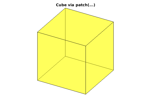
Wuerfel via patch

Create six rectangular faces, each having four vertices, by specifying the x-, y-, and z-coordinates of each vertex:

clear, clc, clf

verts = [ 0 0 0; ...              % the 8 vertices of th cube
          1 0 0; ...
          0 1 0; ...
          1 1 0; ...
          0 0 1; ...
          1 0 1; ...
          0 1 1; ...
          1 1 1 ];

faces = [ 1 2 4 3; ...           % the 6 faces of the cube
          5 6 8 7; ...
          1 2 6 5; ...
          2 4 8 6; ...
          4 3 7 8; ...
          3 1 5 7 ];

patchinfo.Vertices = verts;
patchinfo.Faces = faces;
patchinfo.FaceColor = 'y';          % 'w' for white

patch(patchinfo);

view([30,30])
alpha(0.4)
axis equal
axis off
title('Cube via patch(...)')

Wuerfel via 'box on'

clear, clc, clf
%
plot3([0,1],[0,1],[0,1],'.')           % unsichtbare Diagonale des Wuerfels
box on
axis equal
xlabel('x'),ylabel('y'),zlabel('z')
title('Cube via box on')

You have publish manually from the command window in case of figures

see MATLAB answers.

publish('v_6_a.m');

Published with MATLAB® R2019a